Week 5: Closure#
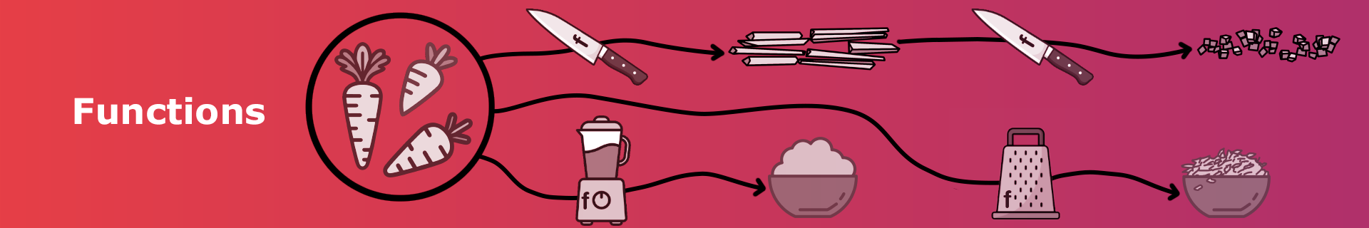
Syllabus Week 5: Functions#
Functions, keyword
defFunction names and naming convention
Function parameters (names given by the function definition)
Function arguments (values passed to the function when called)
Function body and indentation
Calling functions
Variable scope
Returning values, keyword
returnFruitful and void function, side effects,
NonetypeFunction examples: build-in functions, functions included in the standard Python library, functions from common third-party libraries, user-defined functions.
Tracebacks in error messages
Good practice when writing functions (start by scripting, incremental development, scaffolding)
Testing functions
Writing tests for functions
Documenting functions
Advanced#
Some additional concepts to familiarize yourself with are:
Advanced 5.1: Fibonacci Sequence with Recursion#
Hint
You will probably need 3 variables to keep track of the numbers. You can start with f=0 f_next=1 and f_next_next=1. Then you can update the variables in a loop.
Fibonacci with recursion
Recursive functions are functions which call themselves. An example of a recursive implementation of the factorial is included below. How many times is the function called if you want to calculate the factorial of 5? Consider adding a print statement to the function to see how many times it is called.
def factorial(n):
    if n == 0:
        return 1
    else:
        return n * factorial(n-1)
Now, write a recursive function fibonacci_recursive that takes \(n\) as an input and returns the \(n\)th number in the Fibonacci sequence. The function should use recursion to calculate the numbers in the sequence (not a loop).
Advanced 5.2: More About Divisions#
The following exercises use the is_divisible function from the In-Class exercises.
Printing all factors
A factor is a number that divides another number without leaving a remainder. Given a number, we want to know all the numbers that are factors of that number. For example, take the number 12. Looking at all numbers from 1 to 12, we see that 12 is divisible by 1, 2, 3, 4, 6, and 12.
Use is_divisible function to write a function all_factors that takes num as input and prints all the factors of num. For example all_factors(12) should print
1
2
3
4
6
12
Number of times divisible
We want to extend the is_divisible function to return the number of times a number is divisible by another number. For example take the number 12 and divisor 2. If we divide 12 by 2, we get 6, and if we divide 6 by 2, we get 3, which is not divisible by 2. Therefore, 12 is divisible by 2 two times.
Use is_divisible function to write a function num_times_divisible which should alto take two arguments num and divisor. If num is not divisible by divisor, the num_times_divisible function should return 0. If num is divisible by divisor, the function should return the number of times num is divisible by divisor. For example, num_times_divisible(12, 2) should return 2.
Advanced 5.3: Prime Numbers and Factorization#
Also these exercises continue the theme of divisibility.
Is prime
Write a function, is_prime which returns True when a num is prime and False if not. You may have code from a previous week that does this, consider reusing this in the function. If not, a prime number is defined by having only two factors, 1 and itself. So for example, is_prime(7) should return True since 7 is not divisible by 2,3,4,5 and 6. is_prime(6) should return False since 6 is divisible by 2 and 3. A small note: 1 is not a prime number since it only has one factor.
Print prime factors
Any number can be written as a product of prime numbers. For example, \(12\) can be written as \(2 \cdot 2 \cdot 3\), \(13\) can be written as just \(13\) (because it is prime), \(14\) can be written as \(2 \cdot 7\), and so on. Write a function that takes a number as an argument and prints all the prime factors of that number. Feel free to use previous functions you have written. If everything has went well, print_prime_factors(12) should print
2
2
3
and print_prime_factors(13) should print
13
and print_prime_factors(72) should print
2
2
2
3
3
Advanced 5.4: Default Arguments, Positional, and Keyword Arguments#
Default arguments is a way to set a value for an argument if the function is called without that argument. For example, consider the following function which approximates the square root of a number using Newton’s method
def approximate_square_root(x, epsilon=1e-6, max_iter=100, guess=1.0):
    print("Arguments:\nx:", x, "epsilon:", epsilon, "max_iter:", max_iter, "guess:", guess)
    converged = False
    for i in range(max_iter):
        if abs(guess**2 - x) < epsilon:
            converged = True
            break
        guess = (guess + x / guess) / 2
    if not converged:
        print("Did not converge in", max_iter, "iterations. epsilon:", epsilon)
    return guess
print("Actual sqrt(2) = ", 2**0.5)
print("result:",approximate_square_root(2, 1e-6, 100, 1.0))
print("result:",approximate_square_root(2))
print("result:",approximate_square_root(2, 1e-15))
print("result:",approximate_square_root(2, 1e-15, 2))
In the function above, epsilon has a default value of 1e-6. For all the arguments we have:
xhas no default value, so it must be provided when calling the function.epsilonhas default value1e-6.max_iterhas default value100.guesshas default value1.0.
A keyword argument is when you pass an argument with a keyword and a value, like epsilon=1e-6. For example, in the code above, try calling the following
print(approximate_square_root(2, epsilon=1e-10))
print(approximate_square_root(2, max_iter=1000))
print(approximate_square_root(2, guess=100, max_iter=2))
print(approximate_square_root(max_iter=1, x=2))
The keyword notation allows you to pass the arguments in any order, as long as you specify the keyword. If there is a default value, you can also omit the argument (e.g. we don’t need to pass epsilon if we want to use the default value).
A positional argument is when you pass an argument without a keyword, like 2. For example, approximate_square_root(2, 1e-10, 5, 1) only uses positional arguments. Try calling the following (it should give an error!):
print(approximate_square_root(2, guess=1.0, 1e-10))
Python does not allow positional arguments after keyword arguments. This is because it can be ambiguous which argument is which. Python cannot guess if you want 1e-10 to be epsilon or max_iter. You also get an error if you try to pass the same argument twice:
print(approximate_square_root(x=2, x=3))
Advanced 5.5: Global Variables#
In the preparation, you have seen that you can use global variables. In this course, you should avoid using global variables. Try this code to see how it can be rather confusing to figure out what can be changed and what cannot. First run the code as-is. Then, try uncommenting first the one, and then the second commented line. Lastly, try uncommenting both lines.
some_number = 10

def some_function():
    # some_number = 3
    print(some_number)
    a = 5 + some_number
    # some_number = 14
    return a

k = some_function()
print(k)
print(some_number)
Advanced 5.6: Order of Defining Functions#
When you define a function, you can’t call it before it’s defined. This is because Python reads the code from top to bottom. If you try to call a function before it’s defined, you’ll get an error. Here is an example. Fix the code so that it runs without errors.
display_sad_message()
def display_sad_message():
    print("aw man D:")
For functions that call other functions, you can actually define the functions in any order as long as they are all defined before you call any of them. Here is an example.
def calc_kinetic_energy(mass,distance, time):
    velocity = calc_velocity(distance, time)
    kinetic_energy = 0.5 * mass * velocity ** 2
    return kinetic_energy
# calc_kinetic_energy(1,2,3) # This should raise a an error
def calc_velocity(distance, time):
    return distance/time
print("The kinetic energy is:", calc_kinetic_energy(1, 2, 3))
Try to run the code (it should work unchanged). Try to uncomment the line with # and see what error you get.
Advanced 5.7: Naming Functions#
An important aspect of writing functions is to name them appropriately. For example, consider a function which calculates the volume of a cone. A good name for this function would be cone_volume. This name is descriptive and tells you what the function does.
def cone_volume(radius, height):
    pi = 3.141592653589793
    return pi * radius**2 * height / 3
Note that the function name is in lowercase and uses underscores to separate words. This is the convention in Python, however it is not a strict rule and if you want to be different you could name your function ConeVolume, coneVolume or cONeVoLUme but it would likely confuse other Python programmers.
A bad name for this function would be cone, vol or func since these functions don’t describe what it does appropriately. Sometimes it is useful to add a prefix to the function name to indicate what action the function does. The function above could be named calc_cone_volume. Other useful prefixes could be:
print_XXXordisplay_XXX: If your function prints something.calc_XXX,estimate_XXX, orget_XXX: If your function calculates something and/or returns it.update_XXXorchange_XXX: If your function updates or modifies something.check_XXX,is_XXXorhas_XXX: If your function checks something (i.e. returnsTrueif what it checks is true andFalseotherwise).
Match the following functions with an appropriate prefix:
def volume(vol):
    print("My volume is", vol)

def right_triangle(a,b,c):
    return a**2 + b**2 == c**2

def triangle_type(a,b,c):
    if a == b == c:
        return "equilateral"
    elif a == b or b == c or a == c:
        return "isosceles"
    else:
        return "scalene"
Solution
volume->print_volumeordisplay_volumeright_triangle->check_right_triangleoris_right_triangletriangle_type->get_triangle_type
Advanced 5.8: Central Number#
Given three numbers, we want to know which one is the central number. When the three numbers are all different, the central number is the one that is neither the largest nor the smallest. If two or more of the numbers are the same, the central number is that number.
Write a function central_number(a, b, c) that takes three numbers as arguments and returns the number which is central.
Advanced 5.9: Greatest Common Divisor#
The greatest common divisor (GCD) of two numbers (non-negative integers) is the largest number that divides both numbers. For example, the GCD of 12 and 18 is 6. Write a function greatest_common_divisor that takes two numbers as arguments and returns GCD. This is useful if you want to simplify a fraction. For example, the GCD of 12 and 18 is 6 and therefore
If your implementation is correct, then you should expect the results shown in the table below.
num1 |
num2 |
GCD |
|---|---|---|
12 |
18 |
6 |
10 |
15 |
5 |
1024 |
192 |
64 |
100 |
1000 |
100 |
1000 |
100 |
100 |
23 |
23 |
23 |
Consider the following code. It specifically tests the first example from the table above.
expected = 6
output = greatest_common_divisor(12, 18)
if output != expected:
    print("FAILED the following test:")
print("greatest_common_divisor(12, 18) returned", output, "should be", expected)
A complete test of all the expected outputs from the table is available in test_greatest_common_divisor.py. Download this file, then run the test function to test your code. Make sure it imports the function from your file greatest_common_divisor.py. It will only work if
your file is called
greatest_common_divisor.py,your function inside the file is called
greatest_common_divisor,the files
greatest_common_divisor.pyandtest_greatest_common_divisor.pyare in the same directory.
Advanced 5.10: Falling Ball Simulation#
In this exercise, you’ll simulate how long it takes a ball to fall from a certain height to the ground, both with and without air resistance. While this can be solved analytically, we’ll use a simulation based on time steps and a loop. Our final goal it to write a function that takes the initial height of the ball and the time step as arguments and returns the time it takes for the ball to hit the ground. Optionally, the function should also take a constant for air resistance as an argument, and if this is provided it should be used in the simulation. We suggest first writing a script that performs the simulation, and then turning it into a function.
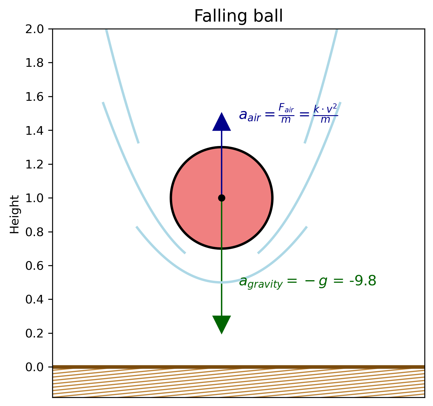
Once dropped, the ball is affected by gravity which accelerates it downwards
and air resistance which opposes motion
where \(r\) is a constant depending on the ball and air properties.
During simulation, you should keep track of the four values: acceleration (in \(\mathrm{m/s}^2\)), velocity (in \(\mathrm{m/s}\)), height (in meters) and the total time passed (in seconds). In each step of the simulation:
compute acceleration based on the previous step \(a_\mathrm{new} = -g + r \, v_\mathrm{old}^2\),
update velocity based on acceleration \(v_\mathrm{new} = v_\mathrm{old} + a_\mathrm{new} \cdot \Delta t\),
update height based on velocity \(h_\mathrm{new} = h_\mathrm{old} + v_\mathrm{new} \cdot \Delta t\),
update time \(t_\mathrm{new} = t_\mathrm{old} + \Delta t\).
You should initialize the variables for acceleration, velocity, height and time to appropriate values and update them in a loop. The loop should run until the height is less than or equal to zero. The value \(\Delta t\) should be set appropriately, for example to 0.01 seconds.
Try to simulate the fall from a height of 1 meter without air resistance. Choose a small time step, like 0.01 seconds. Compare your result to the analytical solution which is \(\sqrt{2h_0/g}\). Add air resistance (e.g. \(r = 0.1\)) and confirm that the fall takes longer. When you are satisfied with your code, wrap your simulation in a function that accepts \(h_0\), \(\Delta t\) and optionally \(r\).
Compare your results with the values we provide below.
>>> falling_ball_simulation(1.0, 0.01)
0.45000000000000023
>>> falling_ball_simulation(100.0, 0.01)
4.519999999999948
>>> falling_ball_simulation(5.0, 0.1, 0.2)
1.2
>>> falling_ball_simulation(3.0, 0.01, 0.1)
0.8200000000000005
>>> falling_ball_simulation(10.0, 0.05, 0.15)
1.800000000000001
falling_ball_simulation.pyfalling_ball_simulation(h0, dt, r)
Calculate the time it takes for a ball to fall.
Parameters:
|
|
Initial height (m). |
|
|
Time step for the simulation (s). |
|
|
Air resistance constant. Defaults to 0. |
Returns:
|
Time it takes for the ball to fall (s). |